
Additional contribution by: Santanu Chatterjee, Trystan Leftwich, Bryan Naden.
In the previous post we demonstrated how to model percentile estimates and use them in Tableau without moving large amounts of data. You may ask, “how accurate are the results and how much load is placed on the cluster?”. In this post we discuss the accuracy and scaling properties of the AtScale percentile estimation algorithm.
Accuracy
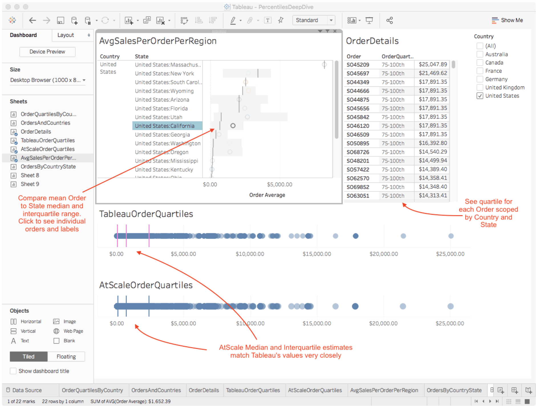
Figure 10. Order Dashboard with Country, State Median Interquartile Range and Order Labels
Figure 10 shows Tableau’s computations of Order Quartiles compared to AtScale’s accuracy estimates. As you can see AtScale’s estimate of the 25th, 50th, and 75th percentiles almost perfectly align the exact calculations performed by Tableau in-memory. To conform to Tableau’s dataset specifications, we restricted the analysis in Figure 10 to a dataset of only 64,000 rows. In reality, we can’t move a whole data-lake into a Tableau data extract, so we stepped outside of Tableau to measure the accuracy characteristics of the AtScale algorithm.
To see how accurately AtScale estimated various percentile thresholds from both symmetrical and skewed datasets, we generated 1 billion row datasets from the normal and gamma distributions (Figure 11). Recall that the “accuracy factor” is the setting that controls how detailed of a histogram AtScale constructs under-the-hood. We wanted to see how well the various accuracy factor settings worked for estimating the 5th, 25th, 50th, 75th, and 99th percentiles of the two different distributions. The low, medium and high “Quality” settings in AtScale’s user interface correspond to “Accuracy Factor” values of 50, 200, and 1000 in our reported results. Additionally, we experimented with values up to 15,000 in an attempt to crash Impala with our UDF.
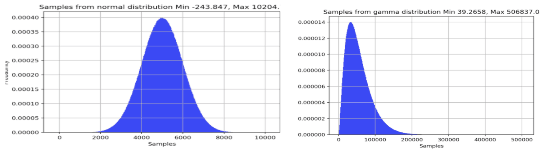
Figure 11. Examples of Normal and Gamma Distributions
Figure 12 displays our accuracy results as error percentages for the two distributions on a logarithmic scale. As expected, larger accuracy factors generally produce estimates with lower error. I’ve drawn a line at an error level of 0.1% as a subjective reference on the log chart. The overall accuracy of most of the settings is quite good, falling below the 0.1% level for most accuracy settings and at most points in the distributions. Only a setting of 50 (“low” UI setting) produces results with an error as high as 0.1%, and this happens only occasionally. For many applications an error rate of 0.1% is perfectly acceptable, however if you require greater accuracy you have the option to reduce the error rate by another three orders of magnitude. For instance, the “high” setting of 1000 consistently estimates with less than 0.001% error on normally distributed data. On the skewed dataset the “high” setting of 1000 produced estimates with less than .005% error on all points except the 5th percentile (0.02% error). Finally, the higher accuracy factor values 5000 – 15000 produced estimates with less than 0.0001% error on most points of the distributions.
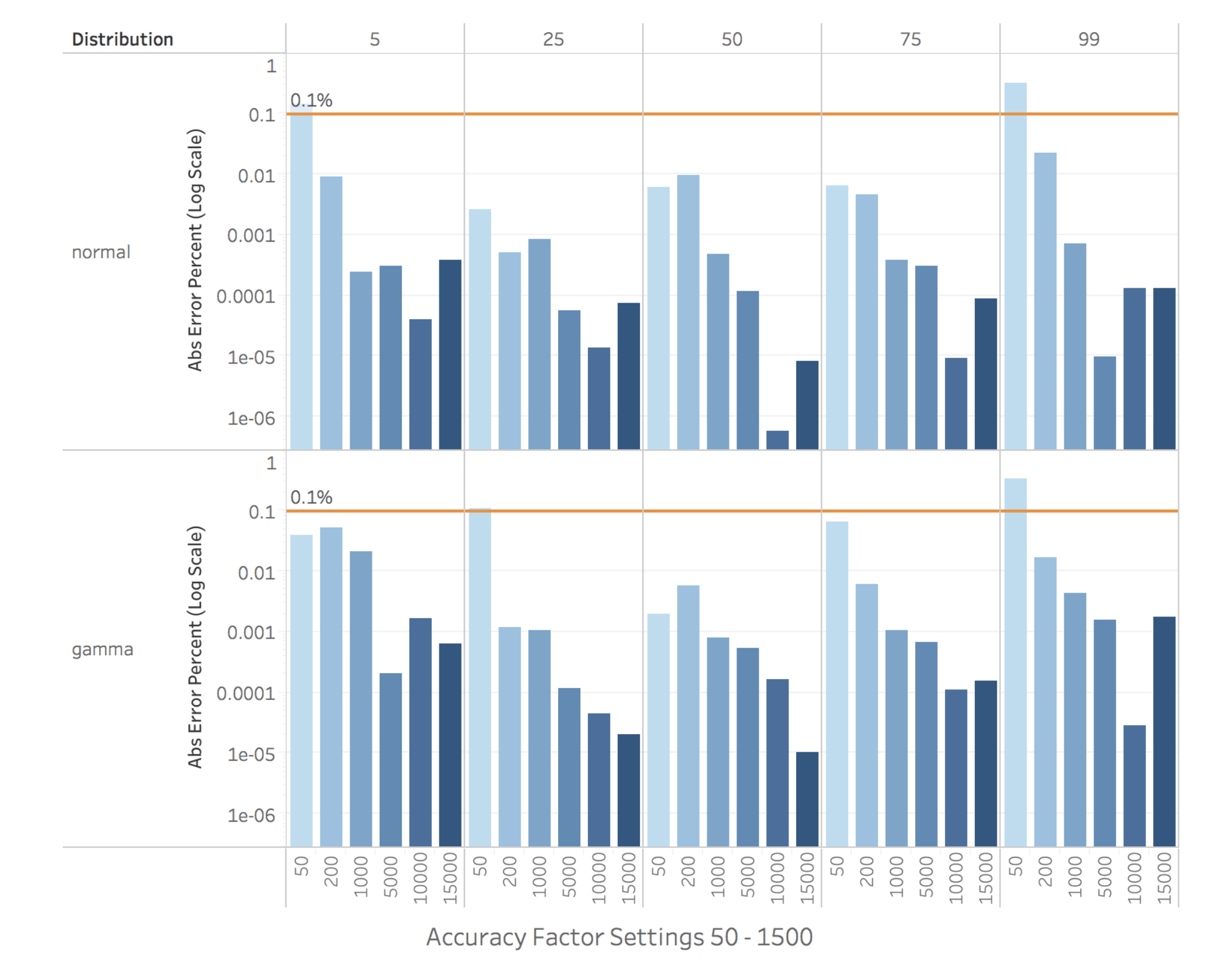
Figure 12. Percentile Estimation Error by Accuracy Factor
Clearly AtScale’s percentile estimation algorithm produces accurate results on large datasets with both symmetric and skewed distributions. But how fast is it and how much cluster memory does it use? In the next section we discuss the memory and time costs of the algorithm by using the tpc-ds benchmark dataset (8.3 billion rows).
Get a better understanding of the data strategies that work and don’t work.
Performance
When developing a new aggregation function we want to understand how the algorithm behaves in a real-world situation running against a large amount of data. The objectives of our performance testing were as follows.
Objectives
- Measure the time and memory cost of running the algorithm.
- Test use-cases that put different workloads on the cluster.
- Test the three typical classes of AtScale queries:
a. inbound queries that don’t hit aggregates,
b. inbound queries that do hit aggregates, and
c. queries that build aggregates - Test the limits of Impala by using extremely high accuracy factor settings.
The Dataset and Model
For this test we selected the tpc-ds dataset, which is an industry-standard decision support benchmark commonly used to measure query performance. AtScale uses this dataset to benchmark the performance of various SQL-on-Hadoop engines. We used the tpc-ds toolkit to generated 8.3 billion rows of sales data. A detailed description of the test schema can be found here. We built an AtScale cube on top of the dataset and exposed the fact table and dimensions need by the test queries.
The Queries
After the model was built, we connected Tableau to AtScale and created three test queries. The query descriptions and pseudocode are as follows:
1. Query 1 - Compute Decile Thresholds:
Select Avg Store Revenue, Store Revenue Deciles group by Country, State, Year, where Country = “US” and State=”CA”
2. Query 2 - Compute Decile Threshold Labels:
Select Avg Store Revenue, Avg Store Revenue Decile Label group by country, state, Customer Dependents where Country=”US” and year = 2003
3. Query 3 - Filter results by Percentile Threshold:
Select US Stores, City, Country with 2003 Avg Sale >= US 2003 90th Percentile
The Cluster
For the test we used a cluster with the following specification:
- 10 nodes
- Node Config: 128G memory, and 32 CPUs, commodity SSDs
- Impala uses 120G of memory per node
- Single-rack, 1GB network
We used a jdbc session parameter max_row_size=8mb to accommodate the large intermediate result set size produced by the test queries. See max_row_size for more information.
Dependent Variables
After executing our test queries we collected the following dependent variables from the Impala query profile. These metrics are the best way we found to quantify the cluster resources used by the algorithm.
- Time (Seconds) – the total time to execute the query
- Max Final Aggregate Task Memory – the max memory reported while handling AtScale’s custom aggregation function
- Max Streaming Aggregate Task Memory – the max memory for a node on the streaming task
Procedure
We ran each of the test queries three times for every accuracy setting reported below. All results presented in Figures 13 – 15 are the average of three trials. AtScale’s query cache was disabled for all tests.
Test 1 – “No Aggregates”
a. Disable aggregate table usage and generation
b. Run all queries against AtScale’s SQL interface (one at a time)
c. Record stats from the query profile
Test 2 – “Use Aggregates”
a. Enable aggregate table usage and generation
b. Execute queries and allow AtScale to generate system-        defined aggregate tables (discard non-agg hit query results)
c. Wait for all aggregate tables to finish populating
d. Run all queries against AtScale’s SQL interface (one at a time)
e. Record stats from the query profile
Test 3 – “Build Aggregates”
a. Enable aggregate table usage and generation
b. For each Test Query (run one at a time):
  - Execute query and allow AtScale to generate system-defined aggregate tables
  - Record stats from the query profile for the aggregate population query
Results
Figure 13 summarizes the results of Test 1, BI queries that do not hit aggregate tables. Queries 1 and 3 executed in ~20s and required no additional time when run with higher accuracy factors. Query 2 executed on the order of ~400s and showed only a slight growth in execution time when run with higher accuracy factors.
Test 1’s Max Final Memory was recorded in the 20M range for settings 50-1000 and in the 30M range for settings 5000 – 15000. The Max Streaming memory for settings 50-1000 were all less than 8M. The max streaming memory grew rapidly for settings 5000 – 15000, however in the worst case of 15000 for Query 2 the max memory remained under an acceptable level of 40M.
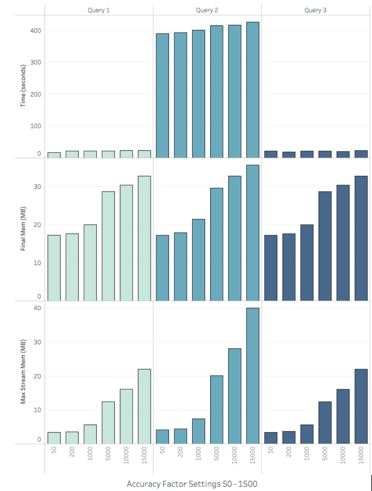
Figure 13. Query Time and Memory by Accuracy Factor (No Aggregates)
Figure 14 summarizes the results of Test 2, BI queries that hit aggregate tables. Queries 1 and 3 executed executed in less than 2 seconds for all accuracy factors and executed in 0.45 and 0.22 seconds when run with an Accuracy Factor of 50 (“low” in the UI). Query 2’s response times are less than 1.5s with accuracy settings 50 and 200, but grow from 20s to 56s when using an Accuracy Factors of 5000 -15000.
Test 2’s Max Final Memory and Streaming Memory metrics showed similar growth characteristics to that of Test 1’s, however they were about 10x larger. This is an expected result because the system is trading CPU and disk IO for memory usage. If computing exact percentiles the cluster would have spent time scanning and sorting individual records. Instead we are using memory to combine fewer (but larger) t-Digest sketches during the reduce steps of the query plan. Although it wasn’t included in this campaign, the max stream and final memory usage can be reduced by turning on AtScale’s Join-in-System-Aggs and Aggregation Partitioning features.
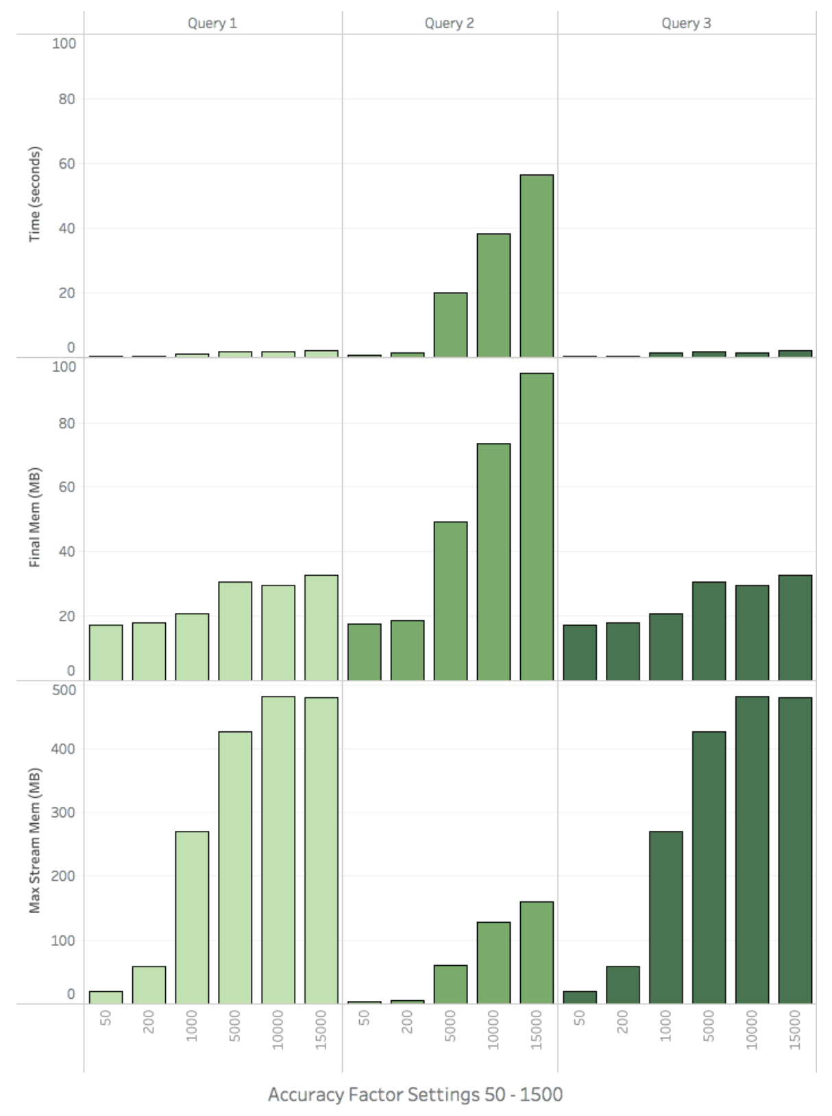
Figure 14. Query Time and Memory by Accuracy Factor (With Aggregates)
Figure 15 displays the results of Test 3, aggregate query build times. As expected the aggregation query times are significantly longer than the inbound query times because these queries have no constraints and therefore process rows for all group-by dimensions. However, for aggregation queries these executed very quickly. For example Query 2 executed in an average of 8.3 minutes using a “high” accuracy factor of 1000.
Final Memory consumption remained less than 120M for all queries when run with an accuracy setting of 50 – 1000. However, the same queries run with accuracy settings 5000 – 15000 rapidly consumed more memory, up to ~1.2G. The growth profile was similar for streaming memory, however the max streaming memory peaked at ~12G.
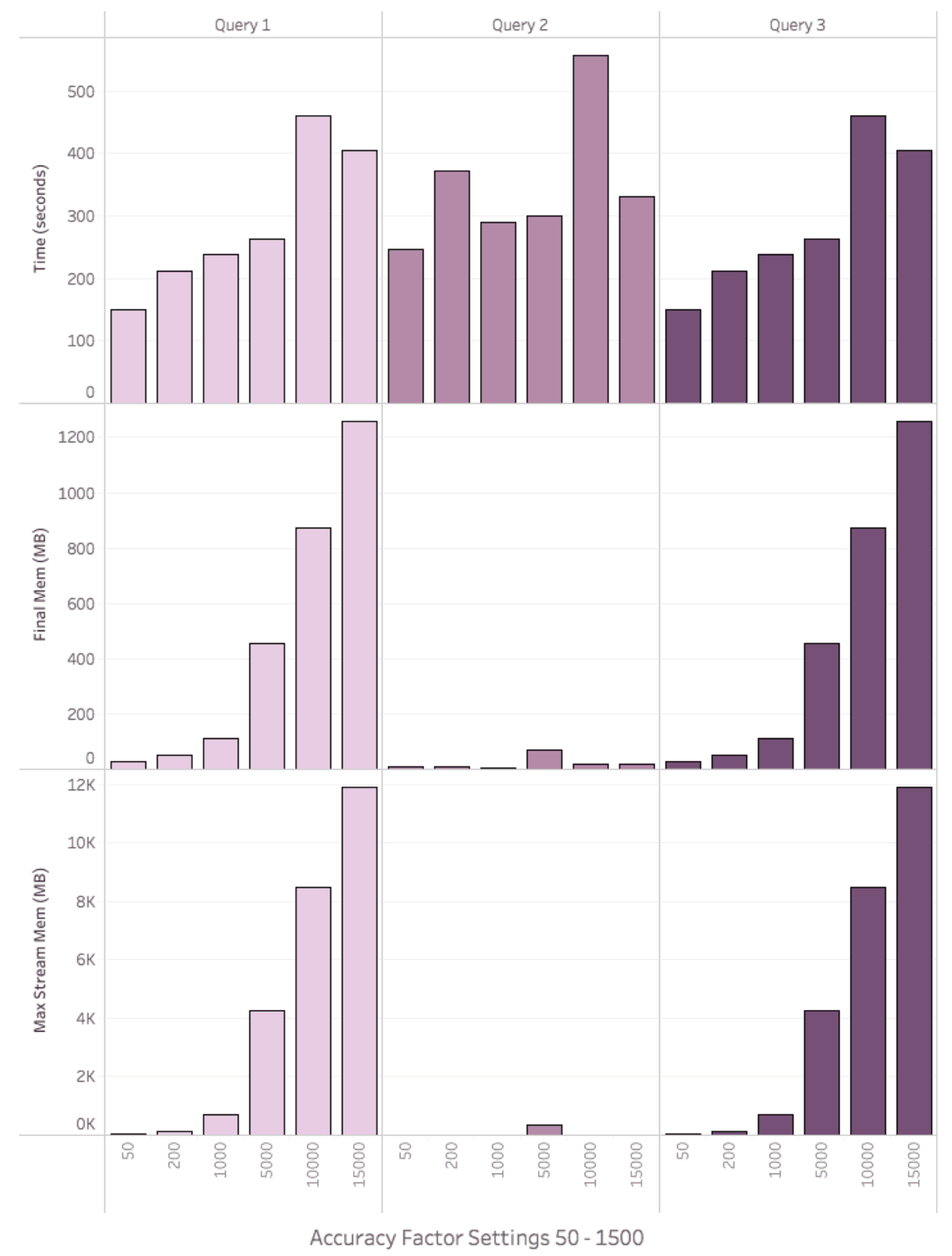
Figure 15. Aggregate Build Time and Memory by Accuracy Factor
Discussion
In most cases accuracy values between 50 – 1000 provided the best accuracy for performance trade-off. This is why in AtScale 6.3 we made the settings 50, 200, and 1000 available as the user-friendly options: low, medium, and high. Because the system did not crash while using larger accuracy settings, we may allow custom values for the “Quality” setting in a future release. If setting a large custom value, one should be mindful of the other queries running on the system. If your workloads call for interactive queries on either symmetrical or skewed data and you can tolerate an error rate of 0.01%, then an accuracy setting of “medium” is a fine trade-off between speed, accuracy, memory consumption, and network usage. Running with “custom” values greater than 5000 to achieve lower error rates without affecting other cluster users may require additional tuning of AtScale settings (i.e. Joins-in-system-aggs, and Aggregate Partitions).
Summary
With this new feature, AtScale delivers unrivaled percentile estimation capabilities that scale to extreme sizes. This leap in performance was made possible by adapting a best-of-breed quantile estimation algorithm to work with AtScale’s semantic layer and adaptive aggregate system. AtScale’s suite of aggregation functions were built from the ground up to work on Big Data. Enterprises no longer have to decide what subset of data they want to analyze because now they can analyze it all.
SHARE
Case Study: Vodafone Portugal Modernizes Data Analytics