Semantic Lakehouse for Business Intelligence
The Databricks Lakehouse combines the best elements of data lakes and data warehouses to deliver the reliability, strong governance, and performance of data warehouses with the openness, flexibility, and machine learning support of data lakes.
The AtScale Semantic Layer stands independent from consumption tools – centralizing governance and control while enabling de- centralized analytics consumption and data product creation.
Removing the Optional Serving Layer and Unleashing the Power of the Lakehouse
AtScale delivers a business-oriented semantic layer that sits on top of the Databricks Lakehouse. AtScale intelligently leverages Databricks to enable users to run low latency BI directly on the Delta Lake.
AtScale drives analytics workloads to Databricks SQL endpoints and clusters to deliver sub second query performance by . automating the creation and maintenance of aggregate tables in Delta Lake.
Organizations spend more time delivering insights and less time maintaining multiple data platforms, maintaining multiple versions of the truth in each and every BI tool.
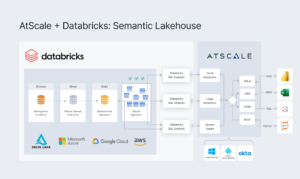
AtScale helps Databricks customers build world-class BI and AI/ML programs while leveraging the full flexibility and capability of Databricks lakehouse.
The AtScale on Databricks Advantage


