Empowering Excel Data Analysis with AtScale: Part 5 – Forecasting

Dave Langer founded Dave on Data, where he delivers training designed for any professional to develop data analysis skills. Over the years, Dave has trained thousands of professionals. Previously, Dave delivered insights that drove business strategy at Schedulicity, Data Science Dojo, and Microsoft. Follow Dave on LinkedIn.

Empowering Excel Analysts

Welcome to the fifth in a series of blog posts showing how AtScale empowers Microsoft Excel users to conduct powerful data analyses.

This blog series is specifically designed for professionals who use Excel. As such, the following principles will guide this blog series:

• The primary focus will be analyzing data using Excel PivotTables.
• Technical details not related to Microsoft Excel will be kept to a minimum.
• Helping Excel PivotTable users learn new features to assist with data analysis.

Throughout this blog series, I will use the term “Excel Analyst” to refer to any professional who analyzes data using Excel PivotTables.

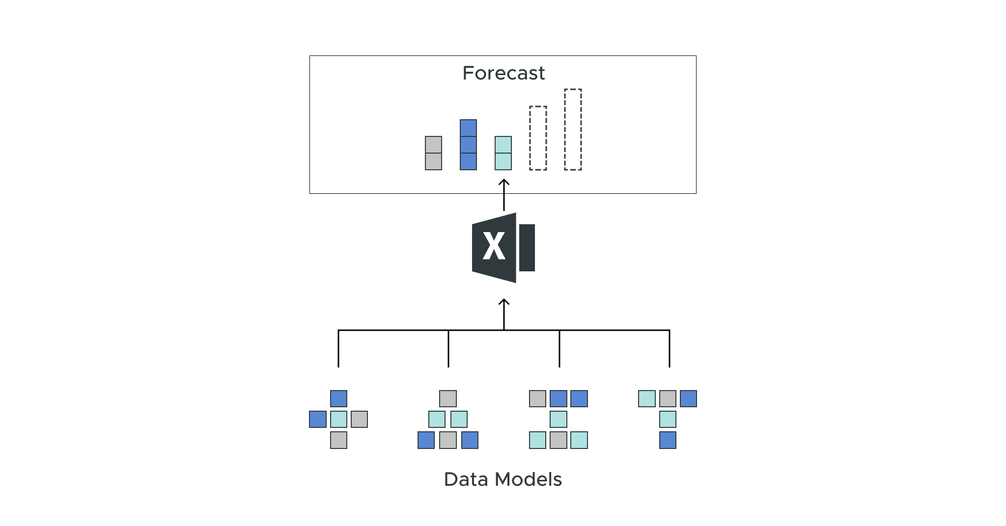
In my experience, the population of Excel Analysts is easily 100+ million professionals worldwide. The goal of this blog series is to help as many of these professionals as possible to achieve more. In this analysis, I use the AtScale Semantic Layer Platform to connect my Excel PivotTables to live cloud data to do high-performing, real-time analysis without any data extraction. Read on to learn how to use Excel PivotTables to forecast data with real-time data without any data extraction.

For convenience, here are links to all the blog posts in this series:

Part 1 – The Scenario
Part 2 – Time Series Analysis
Part 3 – Distribution Analysis
Part 4 – Categorical Analysis
Part 5 – Forecasting (this post)

The Scenario So Far

For a complete description of the hypothetical scenario used in this blog series and for some data background, check out the Part 1 blog post.

At this point in the series, you’ve conducted many analyses into the performance of Internet sales, focusing on understanding the drivers of the Internet Average Order Value (AOV) key performance indicator (KPI).

Your analyses have uncovered the following insights:

• Internet unit sales for mountain and road bicycles have dramatically increased.
• However, the AOV for mountain and road bicycles has steadily declined for years.
• The introduction of miscellaneous products (e.g., bike stands, helmets, clothing, etc.) to Internet sales, while helping drive overall Internet sales growth, has accelerated the decline in AOV.
• The AOV of recently launched touring bicycles has remained consistently higher than mountain and road bicycles.

The next step is to use the knowledge you’ve gained and provide future projections (i.e., forecasts) of Internet sales using the AtScale data model given historical data, assuming no changes are made to the e-commerce business strategy.

Configuring the PivotTable

Using an AtScale data model makes rapidly analyzing data very straightforward because the data model guides configuring your PivotTables:

• Dimensions are used for the rows, columns, and filters of your PivotTables.
• Measures are used for the values of your PivotTables.

This blog post will illustrate using Microsoft Excel’s Forecast Sheet feature with data sourced from a PivotTable.

Adding the Dimension

The Excel Forecast Sheet requires data organized by regularly increasing time intervals. For example, data organized by weeks or months.

Creating forecasts using monthly data is very common because it simultaneously decreases variation (e.g., weekly sales often fluctuate more than monthly sales) while allowing patterns to be detected (e.g., seasonality).

The AtScale data model used in this blog series provides many custom dimensions for representing different timescales (or “grains”) of the data.

In particular, the Order Custom Month Name dimension is useful as it slices the data by a combination of year and month.

The following screenshot shows adding this dimension to the PivotTable.

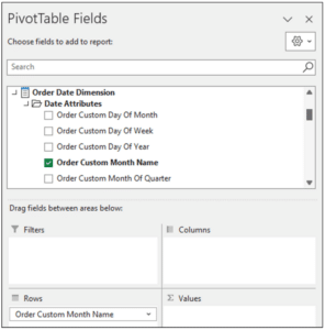
Fig 01 – Adding the Dimension to the PivotTable

The following shows a sample of the Order Custom Month Name data in the PivotTable.

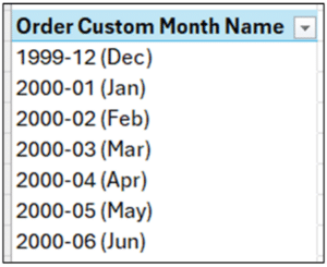
Fig 02 – A Sample of Dimension Data

Adding the Measure

As the Director of e-commerce is under pressure regarding the AOV KPI, the forecasts will focus on this measure.

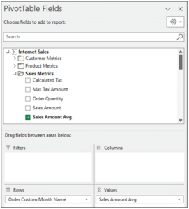
Fig 03 – Adding the Measure to the PivotTable

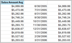
The PivotTable now looks like the following.

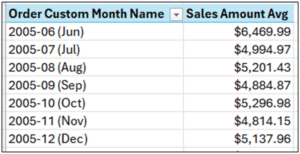
Fig 04 – The PivotTable Data

Adding the Filter

Previous analyses have shown that while the AOV for mountain and road bicycles has declined, these products still represent most Internet sales.

As the future AOV of these two products will greatly impact the overall Internet sales AOV, forecasts focusing on these specific products will provide useful information.

The current PivotTable configuration has aggregated AOV data across all products. Adding the Product Hierarchy dimension as a filter will allow for creating product-specific forecasts.

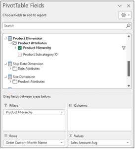
Fig 05 – Adding Product Hierarchy as a Filter

With the PivotTable configured as depicted in Fig 05, the following will filter the AOV data to reflect only mountain bicycles.

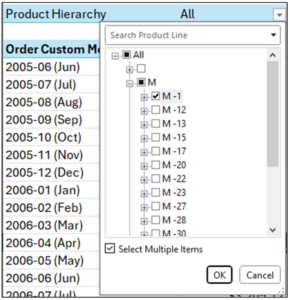
Fig 06 – Filtering AOV to Mountain Bicycles Only

Clicking the OK button on the filter displays the following data in the PivotTable.

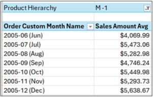
Fig 07 – The Filtered PivotTable AOV Data

The AOV data in Fig 07 is suitable for creating an Excel Forecast Sheet.

Forecasting Mountain Bike AOV

Excel Forecast Sheets are a powerful feature for quickly creating projections of all manner of KPIs (e.g., sales, demand, expenses, etc.).

For the sake of brevity, this blog post will be a simple introduction to Forecast Sheets. For more detailed information, be sure to consult Microsoft’s online documentation.

Preparing the Data

Forecast Sheets have strict requirements regarding the format of the data. Unfortunately, the current PivotTable representations year/month cannot be used.

The easiest solution is to copy and paste the AOV data from the PivotTable to another part of the worksheet.

Fig 08 – Copying and Pasting the AOV Data

The AOV data is aggregated at the monthly level. In other words, the AOV is calculated for the whole month.

Given this, a reasonable approach is to build a forecast based on the last day of each month using the AOV data.

Adding the month-end dates for the first three AOV numbers will allow Excel to understand the date pattern.

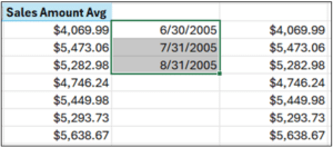
Fig 09 – Adding Dates to the AOV Data

Dragging the selected cell depicted in Fig 09 down the length of the AOV data populates all the required month-end dates.

It’s time to build a Forecast Sheet with the data properly formatted.

The Mountain Bike Forecast Sheet

The first step in building a Forecast Sheet is selecting the date and AOV data.

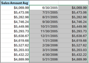
Fig 11 – Selecting the Data for the Forecast Sheet

Next, select Data and then Forecast Sheet from the Excel Ribbon.

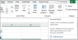
Fig 12 – Accessing the Forecast Sheet Feature

After clicking Forecast Worksheet, the Create Forecast Worksheet dialog will appear. The dialog contains a preview of the forecast.

Clicking on Options in the dialog displays various configuration settings you can set to customize the forecast. This blog post will accept the default options.

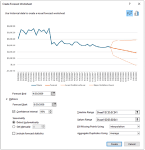
Fig 13 – The Create Forecast Worksheet Dialog

Clicking Create will add a new worksheet to the Excel workbook containing the forecast information, including a line chart of the historical data in blue and the forecasted data in orange.

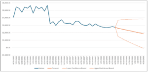
Fig 14 – The Mountain Bike AOV Forecast as a Line Chart

The forecast worksheet also includes detailed data in a table.

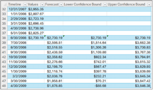
Fig 15 – The Mountain Bike AOV Forecast as a Table

The table depicted in Fig 15 provides a wealth of information:

• The Forecast column shows that, based on historical data, the AOV for mountain bicycles will continue to decline, dropping below $2,000 nine months in the future (i.e., March, 2009).
• Forecasts are never 100% accurate. There is always a level of error. This level of error increases the farther out the forecast.
• The Lower Confidence Bound and Upper Confidence Bound columns provide estimates of likely future AOV values.
• Of particular interest is the Lower Confidence Bound, which forecasts that AOV for mountain bikes could be negative starting in April 2009!

Forecasting Road Bike AOV

Creating a forecast for road bicycles is quite simple, consisting of the following steps as demonstrated above:

• Changing the Product Hierarchy filter to show AOV data only for the R-2 product.
• Copying the AOV values from the PivotTable and pasting over the existing mountain bicycle AOV values in the worksheet.
• Selecting the date and road bicycle AOV data.
• Running the Forecast Sheet feature on the selected data.
• Clicking Create in the Create Forecast Worksheet dialog.

The above steps will add a second forecast worksheet to the Excel workbook.

The Road Bike Forecast Worksheet

The following is the line chart for the road bicycle AOV forecast.

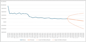
Fig 16 – The Road Bike AOV Forecast as a Line Chart

The following is the table for the road bicycle AOV forecast.

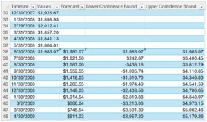
Fig 17 – The Road Bike AOV Forecast as a Table

As with the previous forecast worksheet, the table depicted in Fig 17 provides a wealth of information:

• The Forecast column shows that, based on historical data, the AOV for road bicycles will continue to decline, dropping below $1,000 9 months in the future (i.e., March, 2009).
• The Lower Confidence Bound forecasts that road bicycle AOV could turn negative as soon as August 2008!

The Analysis Results

In business analytics, any analysis aims to explain the “why” of what is happening.

For the hypothetical scenario, here is the “why” of what’s happening in a summarized form suitable for kicking off a data story session with the Director of e-commerce:

The situation:

• Growth of Internet sales has cannibalized Average Order Value (AOV).
• Introducing miscellaneous products (e.g., bike stands, helmets, clothing, etc.) at far lower prices has dramatically reduced AOV.
• The core Internet sales generators of mountain and road bicycles have experienced year-over-year declines in AOV.
• The AOV for these two products is forecasted to continue to decline. Assuming no changes, this trend will have a significant negative impact on Internet sales profitability.

Any good data story should have a recommendation for how to change the situation.

Based on the data analyses, the top priority would be to investigate the causes for the declines in mountain and road bicycle AOV and implement changes to raise the AOV for these products.

Wrap-Up

This blog series demonstrates that combining clean enterprise data from an AtScale data model and Microsoft Excel enables powerful data analyses.

I hope you enjoyed this blog series and developed new data analysis skills.

Until next time, stay healthy and happy data sleuthing!